Introduction
Hello, I’m Hodaka Mori from Preferred Networks. In our previous article, we introduced single-GPU acceleration in our molecular dynamics (MD) code, pfmd, and Batched MD, which runs multiple systems together. Since then, we have expanded support for classical force fields and achieved approximately 10 times the performance of LAMMPS Kokkos for EAM simulations of copper. We can now also run systems of approximately one billion beads on 16 H200 GPUs and two billion beads on 32 H200 GPUs. We have added a command-line interface (CLI) that accepts existing input files and an API for running simulations from Python. We are exploring various possibilities, including making pfmd available externally in the future. Please get in touch if you are interested.
Broader Force-Field Support and Speedups over LAMMPS
The force field required for MD depends on the material or molecule being studied. In pfmd, we have implemented CUDA support for AMBER, CHARMM36, GROMOS 54A7, and MARTINI 3 for proteins and lipids; PCFF for polymers; EAM and MEAM for metals; Stillinger–Weber and Tersoff for covalent crystals; and the reactive force field ReaxFF. We also support polarization with Drude and AMOEBA, and implicit solvent with Generalized Born. Users can now select models suited to their systems, from molecular models with fixed bonding topology to many-body interactions in metals and models that describe bond formation and breaking.
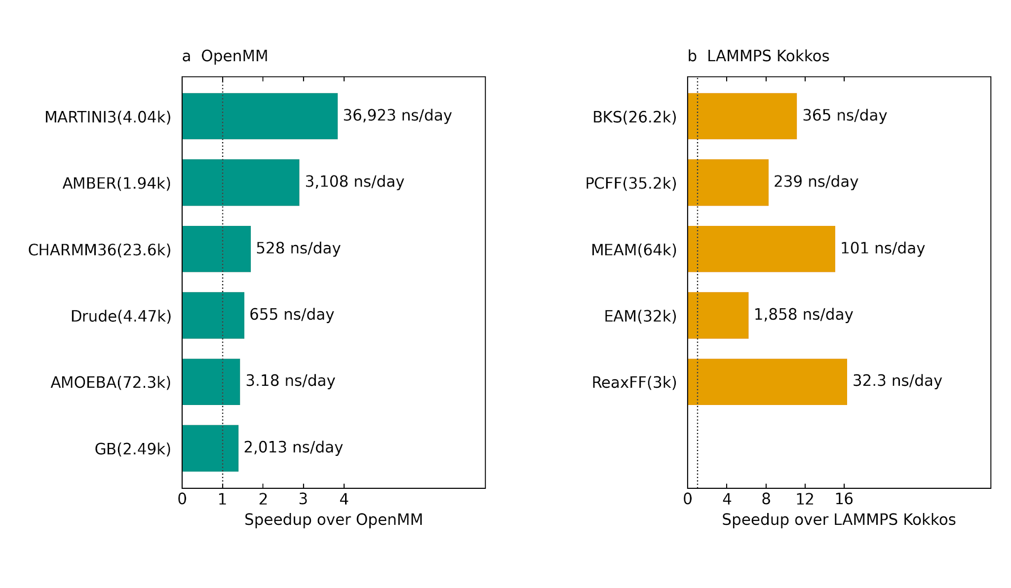
For EAM simulations of copper, pfmd achieved nearly 10 times the performance of LAMMPS Kokkos. We also observed speedups for force fields with different formulations, including PCFF and MEAM. As we added force fields, we retained the design in which time integration and neighbor-list updates run on the GPU. EAM requires the local electron density to be calculated before the forces. We therefore adjusted the data layout, for example to load coordinates and derivatives of the embedding energy together. For ReaxFF, running both bond-order calculations and the iterative QEq calculations that determine atomic charges within CUDA Graphs enabled a speedup of at least 15 times.
Under conditions that yield a nearly tenfold speedup, the time needed to generate a trajectory of the same length falls to approximately one tenth. This makes it possible to compare multiple compositions or temperatures in the time previously spent on a single condition. Expanding the range of systems that can be simulated quickly with suitable force fields also makes it easier to examine how broadly the results apply. Figure 1 shows speedups relative to OpenMM and LAMMPS Kokkos. We report the largest speedup obtained for each force field; benchmark conditions and additional comparisons are given in Appendix A.
Large-Scale Simulations on a Few to a Few Dozen GPUs
Largest Systems Simulated
We have also added multi-GPU and multi-node support to pfmd, allowing a single large system to be simulated across multiple GPUs. We have run all-atom systems with tens of millions of atoms and coarse-grained systems with more than one billion beads on a few to a few dozen GPUs. Handling such large systems requires distributing both computation and data storage. Our distributed implementation divides particles into spatial domains, with each GPU storing its assigned particles and the neighboring particles needed to calculate interactions. Loading of the initial structure and the cells used for neighbor searches are also partitioned by domain, reducing the constraints imposed by having each GPU or host hold the entire system.
For POPC lipid bilayers modeled with MARTINI 3, we ran approximately one billion beads on 16 H200 GPUs and two billion beads on 32 H200 GPUs. With 32 GPUs, throughput reached approximately 12 ns/day for two billion beads and 26 ns/day for one billion beads. All-atom systems can also be distributed while using PME to calculate long-range electrostatic interactions. On eight V100 GPUs, we ran approximately 44 million atoms with AMBER and 36 million atoms with CHARMM36.
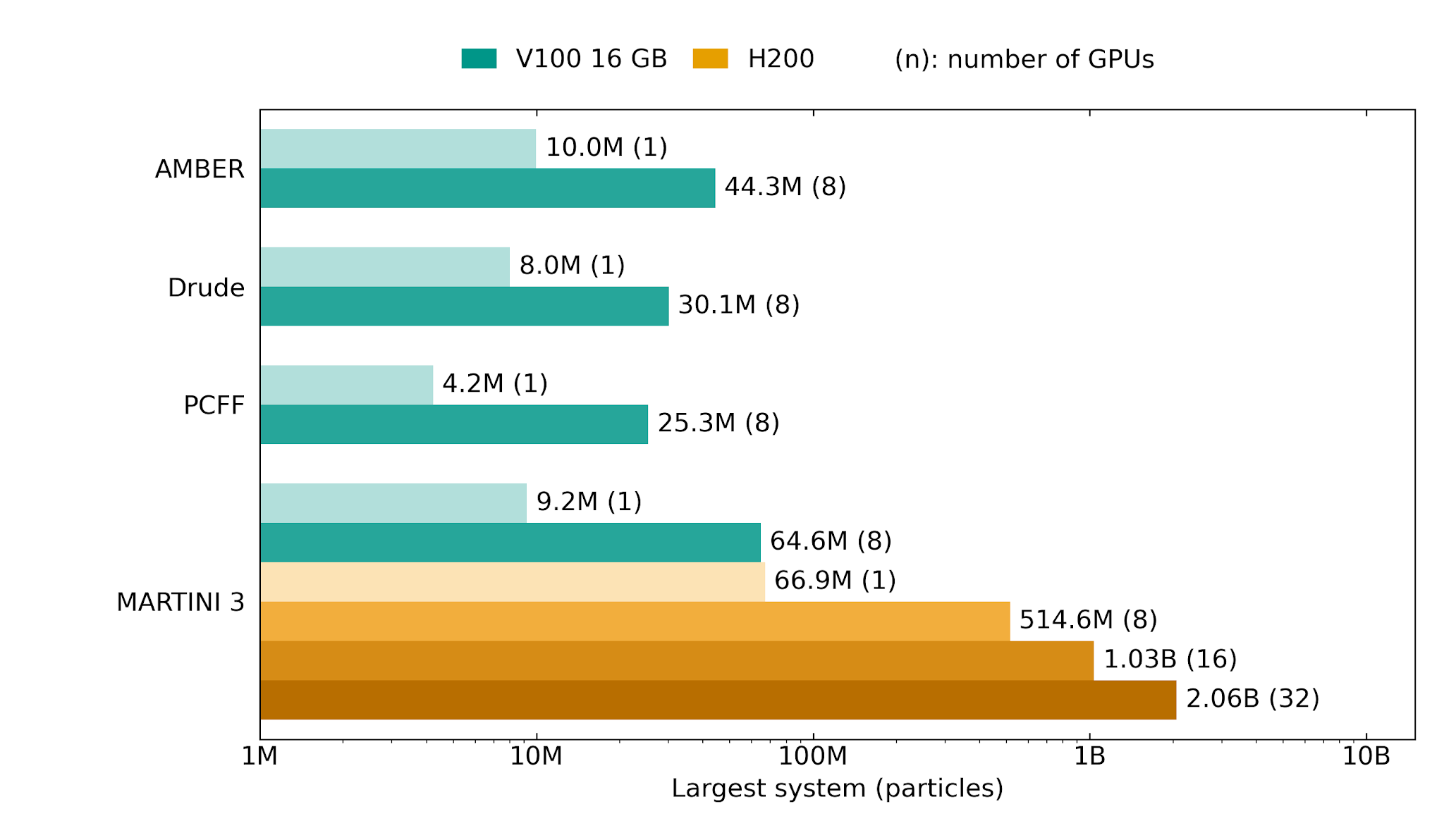
Classical MD has a history of grand challenges that use large fractions of supercomputers to push the limits of system size. TweTriS, reported in 2019 as the world’s largest MD simulation, simulated approximately 20 trillion particles, with a maximum of 21 trillion, using a short-range interaction model [6]. Calculations that include long-range electrostatics have also been reported for approximately 466.1 billion atoms with LAMMPS on Frontier [4] and 1.62 billion atoms with GENESIS for biomolecular systems [3]. With pfmd, we have achieved billion-particle simulations using a few dozen GPUs on a conventional research GPU cluster. The advance here is to make large systems accessible to everyday research without requiring a grand challenge that occupies an entire supercomputer. Benchmark conditions and further context on prior work are given in Appendix B.
The ability to handle a billion particles also broadens the scope for including molecular structure and material heterogeneity in a single model. For example, Sumitomo Rubber Industries simulated filler-containing rubber containing approximately 137 million particles, about 350 nm on each side, on the K computer to analyze void formation and growth after stretching. Those calculations used 7,000 or 28,000 CPU cores [7]. With pfmd, we ran MARTINI 3 lipid membranes containing approximately 515 million beads on eight H200 GPUs and 1.035 billion beads on 16 H200 GPUs. Although the models differ, these results demonstrate simulations on the scale of hundreds of millions of particles on a conventional GPU cluster. This scale provides a starting point for exploring material models that include filler aggregates, polymer chains, and crosslinked networks together. In the life sciences, a single model can similarly encompass multiple membranes, molecular assemblies, and crowded molecular environments, beyond individual proteins or lipid membranes. Coarse-graining brings simulations incorporating organelle or cellular structures, and thus more of the complexity of living systems, within reach. As a concrete example, we ran a simulation of a mitochondrion.
Simulating a Mitochondrion with Approximately One Billion Particles
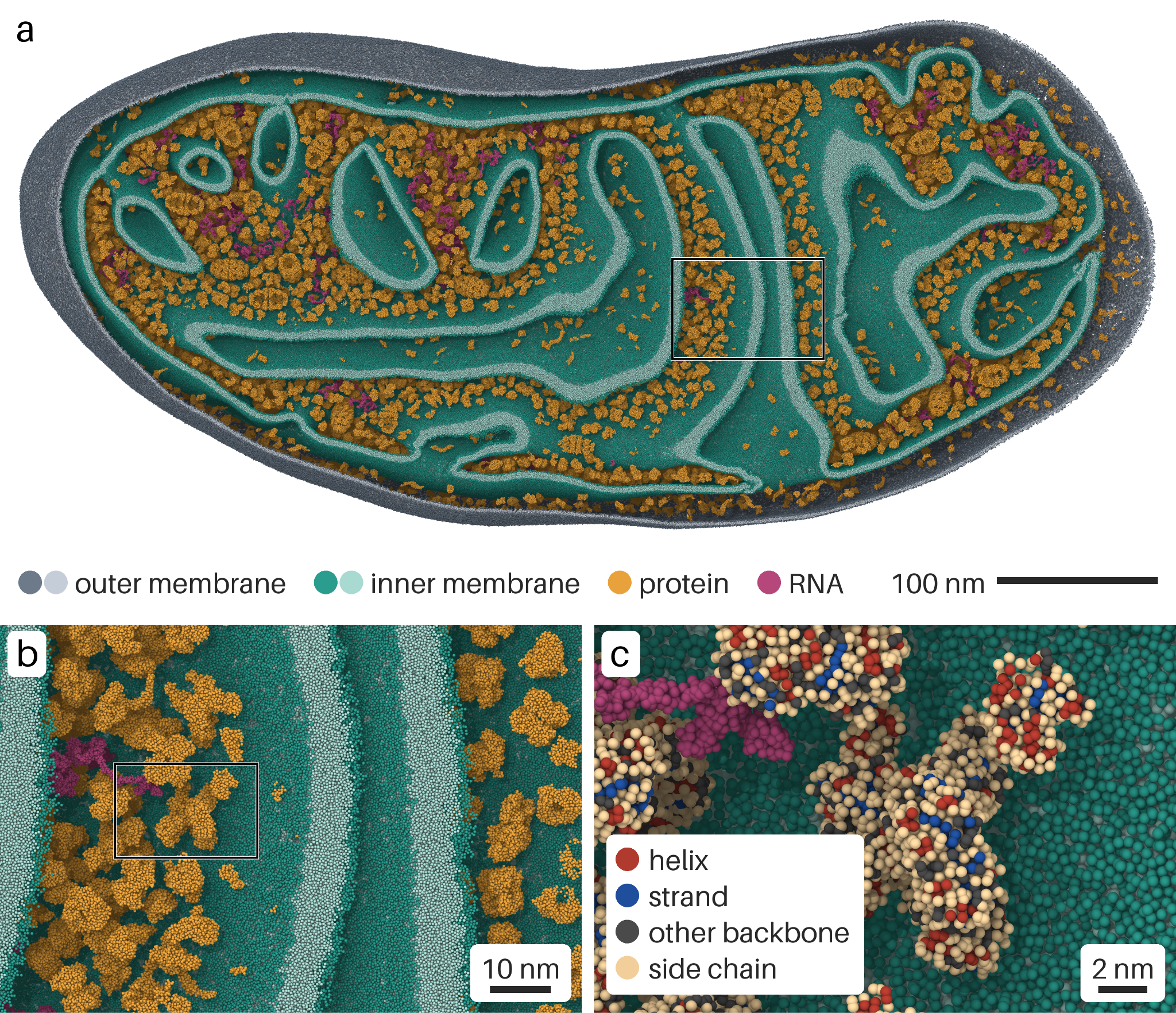
As an application to a large biomolecular system, we used pfmd to simulate a mitochondrial model containing approximately one billion particles, represented as coarse-grained beads. A mitochondrion is enclosed by outer and inner membranes, and the inner membrane forms folds called cristae. We confirmed that MD could be run for a model with this complex geometry. In mitochondria, lipid distributions and membrane-protein arrangements are coupled to membrane shape. Previous work has also reported a coarse-grained model of a crista junction that integrates the inner and outer membranes with multiple membrane proteins [5]. Large-scale MD offers a way to study local molecular interactions and mitochondrial membrane structure within the same model.
Strong Scaling with GPU Count
We also evaluated how much performance improves as GPUs are added while keeping the system size fixed. For a POPC membrane containing approximately 67 million beads, increasing the number of H200 GPUs from one to 32 gave an approximately 30-fold speedup, maintaining a parallel efficiency of about 94%. For AMBER, PCFF, and EAM, increasing the number of V100 GPUs from one to eight yielded speedups of approximately 4.0, 3.6, and 4.7 times, respectively.
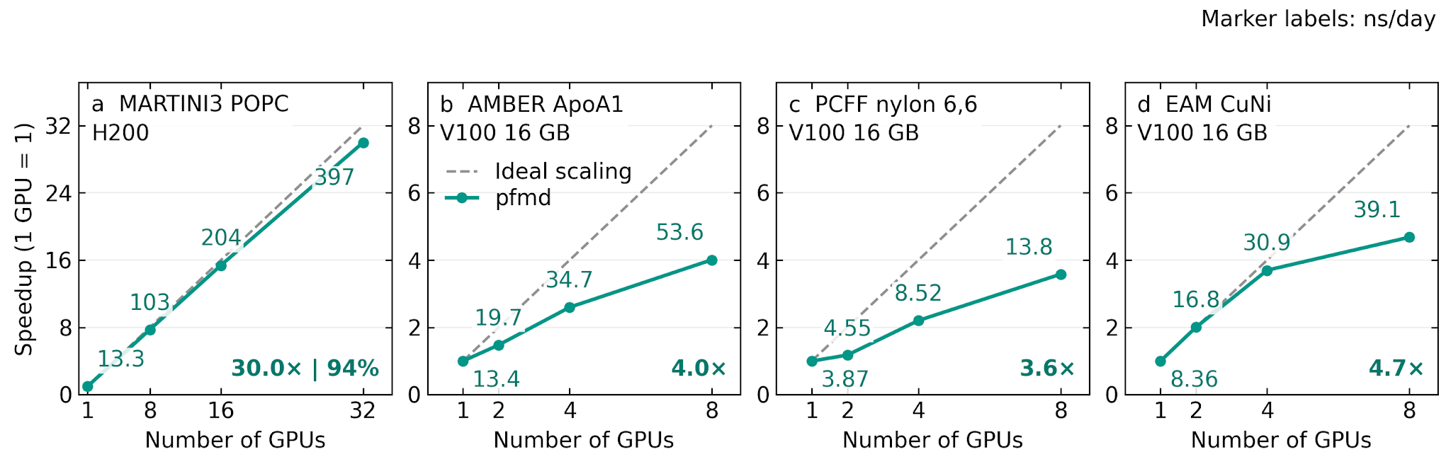
The benefit of adding GPUs depends on system size, so it is important to choose the GPU count to suit the system. There is still room to improve parallel efficiency, particularly for smaller systems or larger GPU counts. Simulating a large system and observing phenomena over long timescales are also separate challenges. A simple extrapolation from the measured 25.8 ns/day for approximately 993 million beads gives about 3.9 days for a 100 ns simulation. This estimate excludes output and operational interruptions. Both the size of the structures of interest and the timescales over which they change need to be considered when comparing compositions or initial structures within the available computational resources. Detailed results for different force fields and system sizes are provided in Appendix C.
Running Simulations through the CLI and Python API
To support reuse of existing research assets, we have added a CLI that accepts LAMMPS and GROMACS inputs, along with a Python API.
A CLI for Existing Input Files
LAMMPS input scripts and GROMACS run-parameter, coordinate, and topology files can be used directly, within the range of supported settings. There is no need to rewrite code for pfmd: users can start from familiar, existing inputs. The following examples run argon and lysozyme systems.
pfmd lmp -i in.argonpfmd gmx -f npt.mdp \
-c gromos-lysozyme.gro \
-r gromos-lysozyme.gro \
-p gromos-lysozyme.topAn API for Running Simulations from Python
The Python API uses syntax similar to OpenMM. Users prepare the system and its force field as a System and pass it, together with an integrator, to Simulation to run MD from Python. Simulation setup and post-processing can be written in Python, while force calculations and time integration run on the GPU. The following example runs a prepared system at 300 K.
from pfmd.integrators import Langevin
from pfmd.sims import Simulation

# The system has already been configured
integrator = Langevin(
    timestep=0.002, temperature=300.0, friction=10.0, seed=42
)
sim = Simulation(system, integrators=[integrator], platform="cuda")
sim.run(50_000)  # 100 ps
The simulation is advanced with sim.run(), and coordinates and energies can be retrieved from Python afterward. For example, a single script can run simulations at several temperatures and pass the results to existing analysis code.
Conclusion
We have expanded and accelerated pfmd’s support for classical force fields and enabled large-scale simulations on a few to a few dozen GPUs. Users can select models suited to molecules, metals, covalent materials, and other systems, while multi-GPU support has increased the system sizes that can be handled. The CLI and Python API allow these simulations to be incorporated into existing research procedures and automated workflows. What matters in research is the ability to simulate a model appropriate to the phenomenon of interest at the required size and timescale. We will continue to expand the supported simulation conditions and improve usability. We are exploring various possibilities, including making pfmd available externally in the future. Please get in touch if you are interested.
Acknowledgments
Some of the calculations presented in this article were performed using ABCI 3.0, provided by the National Institute of Advanced Industrial Science and Technology (AIST) and AIST Solutions.
Appendix: Benchmark conditions and detailed results
A. Force-field performance and benchmark conditions
Representative comparisons in the main text
Figure 1 shows the highest measured speedup for each force field. System sizes may differ between the left and right panels.
The benchmarks used V100 16 GB GPUs, except for EAM and ReaxFF, which used 32 GB GPUs. EAM and ReaxFF were evaluated in the NVE ensemble; the other models used NVT. Force calculations in pfmd generally used single precision, while MEAM and the EAM results in Figure 1 used double precision. OpenMM used mixed precision, and LAMMPS Kokkos used double precision. The BKS and MEAM results in Figure 1 are for α-quartz and 3C-SiC, respectively. AMOEBA used mutual polarization and PME, and ReaxFF used Jacobi QEq. The “nearly 10×” speedup in the main text refers to the 9.97× result for a 32,000-atom EAM system calculated in single precision. The LAMMPS comparison in Figure 1 shows the 6.25× speedup obtained with double precision in both implementations.
Representative measurements
The EAM results in the table were obtained with a V100 32 GB GPU, NVE, and a 5 fs time step; PCFF and MEAM used a V100 16 GB GPU, NVT, and a 1 fs time step. In pfmd, the second EAM row and MEAM used double precision, while PCFF used single precision for force calculations and double precision for integration. EAM values are the medians of three measurements. For PCFF and MEAM, the median of the pfmd timing blocks is compared with the shortest LAMMPS timing block.
For EAM, we also confirmed that the calculated forces agreed with those from the reference implementation.
B. Benchmark conditions for large systems and weak scaling
For MARTINI 3, the POPC membrane was replicated in its plane and simulated in the NVT ensemble at 310 K with a 20 fs time step. Electrostatic interactions were evaluated using the Reaction Field method. The all-atom models were ApoA1 with AMBER and lysozyme with CHARMM36, both using PME for electrostatics. Each H200 node contained eight GPUs.
Performance was measured after warm-up and includes neighbor-list and domain-decomposition updates. Values in ns/day are extrapolated from short timing runs. The maximum particle counts are the largest systems confirmed to run within the implementation and search range used here; equal particle counts do not imply equal computational workloads across models. Weak scaling was evaluated at approximately 31 million beads per GPU, reaching 86.67% efficiency on 32 H200 GPUs. Efficiency is the ratio of the per-step time on one GPU to that on 32 GPUs.
Earlier examples of GPU-parallel MD include approximately 108 million particles on 3,375 GPUs with HOOMD-blue [1] and one billion atoms on 96 V100 GPUs with MDScale [2]. These examples, as well as those discussed in the main text, differ in their models, interactions, and hardware. Particle counts and computing resources are therefore presented as indicators of simulation scale.
C. Detailed strong-scaling results
For strong scaling, the particle count was held fixed while the number of GPUs was increased. Speedup is the per-step time on one GPU divided by the per-step time for each configuration. Parallel efficiency is the speedup divided by the number of GPUs.
The H200 series in Figure 5 uses different timing records from Figure 4a, except for the 32-GPU result. For the POPC membrane with approximately 67 million beads, parallel efficiency reached approximately 94% on 32 H200 GPUs; for approximately 860,000 beads, it was approximately 22% on 16 GPUs.
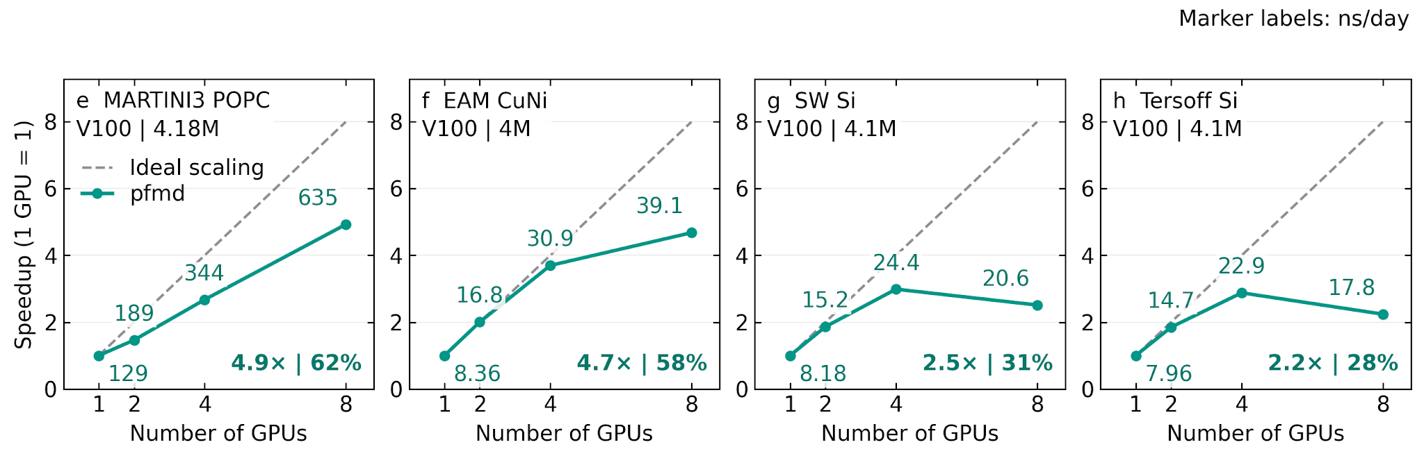
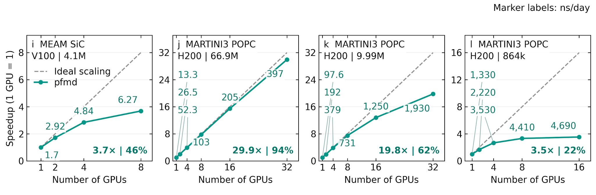
Figure 5. Detailed strong-scaling results. The horizontal axis shows the number of GPUs, and the vertical axis shows speedup relative to one GPU. Dashed lines indicate ideal scaling. Values beside the markers are in ns/day; the bottom-right labels show the speedup and parallel efficiency at the largest GPU count. Panels a–i use V100 16 GB GPUs, and j–l use H200 GPUs. k denotes thousand, M denotes million, and SW denotes Stillinger–Weber. The EAM, Stillinger–Weber, Tersoff, and MEAM implementations store all atoms on each GPU.
References
- J. Glaser et al., Comput. Phys. Commun. 192, 97 (2015).
- G. N. Barreales, M. Novalbos, M. A. Otaduy, and A. Sanchez, J. Parallel Distrib. Comput. 157, 243 (2021).
- J. Jung et al., J. Comput. Chem. 42, 231 (2021).
- N. Hagerty and D. Asthagiri, OLCF-6 LAMMPS Benchmark (2024).
- C. M. Brown et al., Commun. Biol. 8, 972 (2025).
- N. Tchipev et al., Int. J. High Perform. Comput. Appl. 33, 838 (2019).
- M. Naito and H. Kishimoto, Nippon Gomu Kyokaishi 89, 176 (2016).